3. Single Stellar Populations

As discussed in our section on implementation, VICE’s simulations are implemented with a Forward Euler timestep solution, an approximation made possible by numerics not being the dominant source of error. The quantization of timesteps necessitates the quantization of the episodes of star formation. This allows VICE to model enrichment in both singlezone and multizone models by using summations over a sample of discretized stellar populations.

For this reason, we implement a treatment of two quantities particularly useful in the mass evolution of single stellar populations: the cumulative return fraction (CRF) and the main sequence mass fraction (MSMF). The CRF represents the fraction of a single stellar population’s mass that is returned to the interstellar medium as gas. The MSMF is the fraction of its mass that is still in the form of main sequence stars. These quantities are of particular use in calculating the rate of mass recycling and the rate of enrichment from asymptotic giant branch stars.

3.1. Stellar Lifetimes

In VICE we adopt the following functional form for the lifetime of a star on the main sequence:

\[\tau_\text{MS} = \tau_\odot m^{-\alpha}\]

where \(\tau_\odot\) is the sun’s main sequence lifetime, \(\alpha\) is the power-law index of the mass-lifetime relationship. The constant SOLAR_LIFETIME declares \(\tau_\odot\) = 10 Gyr, and MASS_LIFETIME_PLAW_INDEX delcares \(\alpha\) = 3.5. Both constants are declared in vice/src/ssp.h.

The scaling of \(\tau_\text{MS} \sim m^{-3.5}\) fails for high mass stars (\(\gtrsim 8 M_\odot\)), but these stars have lifetimes that are very short compared to the relevant timescales of galactic chemical evolution (\(\sim\)few` Gyr). This approximation fails for low mass stars as well (\(\lesssim 0.5 M_\odot\)), but these stars have very long lifetimes that are considerably longer than the age of the universe. Because VICE does not support simulations on this long of timescales, this approximation suffices for all timescales of interest.

This is motivated by a conventional power-law relationship between mass and luminosity \(L \sim M^{+\beta}\). The lifetime then scales as \(\tau \sim M/L \sim M^{1 - \beta}\). \(\alpha\) = 3.5 corresponds to \(L \sim M^{4.5}\) in the mass range of interest.

This equation can be generalized to find the the total lifetime of a star of mass \(m\): the time until it produces a remnant by simply amplifying the lifetime by a factor \(1 + p_\text{MS}\):

\[\tau_\text{total} = (1 + p_\text{MS})\tau_\odot m^{-\alpha}\]

where \(p_\text{MS}\) is an adopted lifetime ratio of the post main sequence to main sequence phases of stellar evolution.

By interpreting \(\tau_\text{total}\) as lookback time, we can solve for the mass of remnant producing stars under this model.

\[m_\text{postMS} = \left(\frac{t}{(1 + p_\text{MS})\tau_\odot} \right)^{-1/\alpha}\]

This equation allows the solution of both the main sequence turnoff mass and the mass of stars at the end of their post main sequence lifetimes by whether or not \(p_\text{MS}\) = 0.

Relevant source code:

• vice/src/ssp.h

• vice/src/ssp/mlr.c

3.2. The Cumulative Return Fraction

The cumulative return fraction is defined as the mass fraction of a single stellar population that is returned back to the interstellar medium (ISM) as gas. When dying stars produce their remnants, whatever material that does not end up in the remnant is returned to the ISM. This quantity can be calculated from an initial-final mass relation and an adopted stellar initial mass function (IMF). In short, the cumulative return fraction can be stated mathematically as “ejected material from dead stars in units of total initial amount of material.” Its analytic form is therefore given by:

\[r(t) = \int_{m_\text{to}(t)}^u (m - m_\text{rem})\frac{dN}{dm} dm \left[\int_l^u M \frac{dN}{dm} dm\right]^{-1}\]

The current version of VICE employs the initial-final remnant mass relation of Kalirai et al. (2008) 1:

\[m_\text{rem}(m) = \Biggl \lbrace { 1.44\ (m \geq 8) \atop 0.394 + 0.109 m\ (m < 8) }\]

For a power-law IMF \(dN/dm \sim m^{-\alpha}\), the numerator of \(r(t)\) is thus given by:

\[\int_{m_\text{to}(t)}^u (m - m_\text{rem}(m)) \frac{dN}{dm} dm = \frac{1}{2 - \alpha} m^{2 - \alpha}\Bigg|_{m_\text{to}(t)}^u - \frac{1.44}{1 - \alpha} m^{1 - \alpha} \Bigg|_{m_\text{to}(t)}^u\]

for \(m_\text{to}(t) \geq 8\), and

\[\int_{m_\text{to}(t)}^u (m - m_\text{rem}(m)) \frac{dN}{dm} dm = \frac{1.44}{1 - \alpha} m^{1 - \alpha} \Bigg|_8^u + \left[\frac{0.394}{1 - \alpha}m^{1 - \alpha} + \frac{0.109}{2 - \alpha}m^{2 - \alpha} \right]_{m_\text{to}(t)}^8\]

for \(m_\text{to}(t) < 8\).

This solution is analytic. For piecewise IMFs, this becomes a summation over the relevant mass ranges of the IMF, and each term has the exact same form. The normalization of the IMF is irrelvant here, because the same normalization will appear in the denominator.

The denominator has a simpler analytic form:

\[\int_l^u m \frac{dN}{dm} dm = \frac{1}{2 - \alpha} m^{2 - \alpha} \Bigg|_l^u\]

Here we plot \(r\) as a function of the stellar population’s age. Weinberg, Andrews, and Freudenburg (2017) 2 adopted instantaneous recycling, whereby a fraction of the stellar population’s mass \(r_\text{inst}\) is returned instantaneously in the interest of an analytic approach to singlezone models. They find that \(r_\text{inst}\) = 0.4 and \(r_\text{inst}\) = 0.2 is an adequate approximation for Kroupa 3 and Salpeter 4 IMFs. This reduces the more sophisticated formulation implemented here to:

\[r(t) \approx \Bigg \lbrace { r_\text{inst}\ (t = 0) \atop 0\ (t > 0) }\]

In reality, the rate of mass return from a stellar population of mass \(M_*\) is given by \(\dot{r}M_*\), but in implementation, the quantization of timesteps allows each timestep to represent a single stellar population which will eject mass \(M_*dr\) in a time interval \(dt\). For that reason, VICE is implemented with a calculation of \(r(t)\) rather than \(\dot{r}\).

In simulations, VICE allows users the choice between the time-dependent formulation of \(r(t)\) derived here and the instantaneous approximation of Weinberg, Andrews, and Freudenburg (2017) by specifying a preferred value of \(r_\text{inst}\), which allows any fraction between 0 and 1.

In calculations of \(r(t)\) with the built-in Kroupa and Salpeter IMFs, the analytic solution is calculated. In the case of a user-customized IMF, VICE solves the equation numerically using quadrature.

Note

The approximation of \(h(t) \approx 1 - r(t)\) where \(h\) is the main sequence mass fraction fails at the \(\sim5-10\%\) level. See our discussion of this point here.

Relevant source code:

• vice/src/ssp/crf.c

• vice/src/yields/integral.c

1

Kalirai et al. (2008), ApJ, 676, 594

2

Weinberg, Andrews & Freudenburg (2017), ApJ, 837, 183

3

Kroupa (2001), MNRAS, 322, 231

4

Salpeter (1955), ApJ, 121, 161

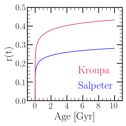
The cumulative return fraction as a function of age for Kroupa 5 (red) and Salpeter 6 (blue) IMFs. The Kroupa IMF is higher at all nonzero ages because it has fewer low mass stars than Salpeter. In both cases the post main sequence lifetime is assumed to be 10% of the main sequence lifetime (i.e. \(p_\text{MS} = 0.1\)).

5

Kroupa (2001), MNRAS, 322, 231

6

Salpeter (1955), ApJ, 121, 161

3.3. The Main Sequence Mass Fraction

The main sequence mass fraction, as the name suggests, is the fraction of a single stellar population’s initial mass that is still in the form of main sequence stars. Because this calculation does not concern evolved stars, neither a model for the post main sequence lifetime nor an initial-final remnant mass relation is needed; it is thus considerably simpler than the cumulative return fraction. This quantity is instead specified entirely by the IMF and the mass-lifetime relation.

It’s analytic form is given by:

\[h(t) = \int_l^{m_\text{to}(t)} m\frac{dN}{dm} dm \left[ \int_l^u m\frac{dN}{dm} dm \right]^{-1}\]

which for a power-law IMF \(dN/dm \sim m^{-\alpha}\) becomes

\[h(t) = \left[\frac{1}{2 - \alpha}m^{2 - \alpha}\Bigg|_l^{m_\text{to}(t)}\right] \left[\frac{1}{2 - \alpha}m^{2 - \alpha}\Bigg|_l^u\right]^{-1}\]

It may be tempting to cancel the factor of \(1/(2 - \alpha)\), but more careful consideration must be taken for piece-wise IMFs like Kroupa 7:

\[h(t) = \left[ \sum_i \frac{1}{2 - \alpha_i} m^{2 - \alpha_i} \right]_l^{m_\text{to}(t)} \left(\left[ \sum_i \frac{1}{2 - \alpha_i} m^{2 - \alpha_i} \right]_l^u\right)^{-1}\]

where the summation is over the relevant mass ranges with different power-law indeces \(\alpha_i\). In the case of kroupa \(\alpha\) = 2.3, 1.3, and 0.3 for \(m\) > 0.5, 0.08 \(\leq m \leq\) 0.5, and \(m\) < 0.08, respectively.

Here we plot \(h\) as a function of the stellar population’s age. By 10 Gyr, \(h(t)\) is as low as \(\sim0.45\) for the Kroupa IMF and \(\sim0.65\) for the Salpeter 8 IMF. In comparison, the cumulative return fraction \(r(t) \approx 0.45\) for the Kroupa IMF and \(\sim0.28\) for the Salpeter IMF. This suggests that the approximation \(h(t) \approx 1 - r(t)\) fails at the \(\sim5-10\%\) level, depending on the choice of IMF. This suggests that for old stellar populations, a non-negligible portion of the mass is contained in evolved stars and stellar remnants. VICE therefore differentiates between these two quantities in its implementation.

In reality, the rate of the stellar mass evolving off of the main sequence is given by \(\dot{h}M_*\) where \(M_*\) is the initial mass of the stellar population. However, the quantization of timesteps in VICE allows each timestep to represent a single stellar population which will eject mass \(M_*dh\) in a time interval \(dt\). For that reason, VICE is implemented with a calculation of \(h(t)\) rather than \(\dot{h}\).

In calculations of \(h(t)\) with the built-in Kroupa and Salpeter IMFs, the analytic solution is calculated. In the case of a user-customized IMF, VICE solves the equation numerically using quadrature.

Relevant source code:

• vice/src/ssp/msmf.c

• vice/src/yields/integral.c

7

Kroupa (2001), MNRAS, 322, 231

8

Salpeter (1955), ApJ, 121, 161

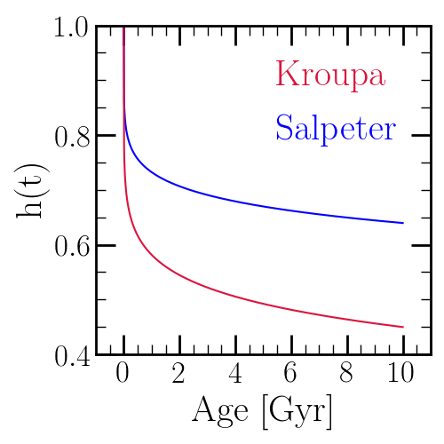
The main sequence mass fraction as a function of age for Kroupa 9 and Salpeter 10 IMFs. The Kroupa IMF is lower at all nonzero ages because it has fewer low mass stars than Salpeter.

9

Kroupa (2001), MNRAS, 322, 231

10

Salpeter (1955), ApJ, 121, 161

3.4. Enrichment from Single Stellar Populations

While galaxies form stars continuously, it is often an interesting scientific problem to quantify the nucleosynthetic production of only one population of conatal stars. This is inherently cheaper computationally, since this is only one stellar population while galaxy simulations require many stellar populations.

VICE includes functionality for simulating the mass production of a given element from a single stellar population (i.e. an individual star cluster) of given mass and metallicity under user-specified yields. This by construction does not take into account depletion from infall low metallicity gas and star formation, ejection in outflows, recycling, etc. It only calculates the mass production of the element as a function of the stellar population’s age.

The star cluster is assumed to form at time \(t = 0\), and thus at this time there is no net production. Because VICE operates under the assumption that all core-collapse supernovae (CCSNe) occur instantaneously following the star cluster’s formation 11, the entire CCSN net yield is injected within the first timestep at \(t = \Delta t\):

\[\Delta M_x = y_x^\text{CC}(Z) M_\star\]

where \(y_x^\text{CC}(Z)\) is the user’s current setting for CCSN yields at a stellar metallicity Z. At subsequent timesteps, enrichment from asymptotic giant branch (AGB) stars is injected according to 12:

\[\dot{M}_x^\text{AGB}\Delta t \approx y_x^\text{AGB}(m_\text{postMS}(t), Z)M_\star \left[h(t) - h(t + \Delta t)\right]\]

and from type Ia supernovae (SN Ia) according to 13:

\[\dot{M}_x^\text{Ia}\Delta t \approx y_x^\text{Ia}(Z) M_\star \frac{ R_\text{Ia}(t) }{ \int_0^\infty R_\text{Ia}(t') dt' }\]

These are the same equations that are implemented in simulating enrichment under the single-zone approximation, but applied to only one episode of star formation.

Users can run these simulations by calling vice.single_stellar_population.

Relevant Source Code:

• vice/src/ssp/ssp.c

• vice/core/ssp/_ssp.pyx

11

See the discussion of enrichment from CCSNe for justification of this assumption.

12

Justification of this can be found here.

13

Justification of this can be found here.

3.5. In Multizone Models

Like the timesteps in singlezone simulations, VICE treats star particles in multizone simulations as stand-ins for entire stellar populations. They eject newly produced heavy nuclei to the interstellar medium and recycle mass at their birth metallicities at the rates detailed in this section, where \(M_\star\) denotes the mass of the star particle.