3. Single Stellar Populations
As discussed in our section on implementation, VICE’s simulations are implemented with a Forward Euler timestep solution, an approximation made possible by numerics not being the dominant source of error. The quantization of timesteps necessitates the quantization of the episodes of star formation. This allows VICE to model enrichment in both singlezone and multizone models by using summations over a sample of discretized stellar populations.
For this reason, we implement a treatment of two quantities particularly useful in the mass evolution of single stellar populations: the cumulative return fraction (CRF) and the main sequence mass fraction (MSMF). The CRF represents the fraction of a single stellar population’s mass that is returned to the interstellar medium as gas. The MSMF is the fraction of its mass that is still in the form of main sequence stars. These quantities are of particular use in calculating the rate of mass recycling and the rate of enrichment from asymptotic giant branch stars.
3.1. Stellar Lifetimes
The simplest description of the relationship between a star’s mass and its lifetime (i.e. the mass-lifetime relationship, hereafter MLR) is a single power law:
where \(\tau_\odot\) is the sun’s main sequence lifetime and \(\alpha\)
is the power law index of the MLR.
The constants SOLAR_LIFETIME and MASS_LIFETIME_PLAW_INDEX, both
declared in vice/src/ssp.h, assign the values of \(\tau_\odot\) = 10
Gyr and \(\alpha\) = 3.5, respectively.
Motivated by a popular exercise in undergradaute astronomy courses, this form
follows from an assumed single-power law relating the mass and luminosity of
stars: \(L \sim M^{1 + \alpha}\).
Because the lifetime of a star scales with its luminosity per unit mass, the
power law then follows trivially: \(\tau \sim M/L \sim M/M^{1 + \alpha}
\sim M^{-\alpha}\).
VICE generalizes this form to describe the total lifetime of a star of mass \(m\) by simply amplifying the main sequence lifetime by a factor of \(1 + p_\text{MS}\):
where \(p_\text{MS}\) is the ratio of a star post main sequence lifetime to its main sequence lifetime (e.g. if the post main sequence lifetime is 10% of the main sequence lifetime, then \(p_\text{MS}\) = 0.1). As a consequence, this quantity describes the time interval between a star’s formation and when it produces a remnant.
By interpreting \(\tau_\text{total}\) as lookback time, VICE solves for the mass of “remnant-producing” stars from a stellar population of known age:
Since these are the stars that are at the ends of the lifetimes, VICE adopts \(m_\text{postMS}\) as written here as the mass of AGB stars enriching the interstellar medium at a given timestep. This equation also allows the solution of the main sequence turnoff mass by simply taking \(p_\text{MS}\) = 0.
The scaling of \(\tau_\text{MS} \sim m^{-3.5}\) fails for higher mass stars (\(\gtrsim 4 M_\odot\)). However, these stars generally have lifetimes that are short compared to the relevant timescales of galactic chemical evolution (\(\lesssim\) 100 Myr compared to \(\sim\) few Gyr). Regardless of its accuracy for low mass stars (\(\lesssim 0.5 M_\odot\)), their lifetimes are considerably longer than the age of the universe anyway, and VICE does not support simulations on timescales longer than 15 Gyr. Consequently, this approximation generally suffices for galactic chemical evolution models.
The important exception to this rule is that an accurate MLR for \(4 \lesssim M/M_\odot \lesssim 8\) stars is necessary when considering elements with significant nucleosynthetic yields from these stars (e.g. nitrogen, Johnson et al. 2021 [1]). Prior to version 1.3.0, VICE implemented this single power law relationship only. In subsequent versions, a handful of additional forms are available to fill this need:
Larson (1974) [2] (default in versions >= 1.3.0)
This form is a metallicity-independent parabola in \(\log\tau-\log m\) space describing the main sequence lifetimes only:
\[\log_{10}\tau = \alpha + \beta\log_{10}m + \gamma (\log_{10}m)^2\]where the original values of \(\alpha\) = 1.02, \(\beta\) = -3.57, and \(\gamma\) = 0.90 were derived from a fit to the compilation of evolutionary lifetimes presented in Tinsley (1972) [3]. VICE however adopts the updated values of \(\alpha\) = 1.0, \(\beta\) = -3.42, and \(\gamma\) = 0.88 from Kobayashi (2004) [4] and David, Forman & Jones (1990) [5]. In detail, the value of \(\alpha\) directly quantifies the log of the main sequence lifetime of the sun \(\log_{10}\tau_\odot\) in whatever units \(\tau\) is in (\(\alpha\) = 1.0 for \(\tau_\odot\) = 10 Gyr; \(\alpha\) = 10.0 for \(\tau_\odot = 10^{10}\) yr).
Solutions to the inverse function (i.e. mass as a function of lifetime) follow directly from the quadratic formula: \(\log_{10}m = (-\beta \pm \sqrt{\beta^2 - 4\gamma(\alpha - \log_{10}\tau)}) / (2\gamma)\). The correct solution comes when choosing subtraction in the numerator as this corresponds to increasing lifetimes with decreasing stellar mass.
This is the default MLR for VICE version 1.3.0 and later.
Maeder & Meynet (1989) [6]
This form is a metallicity-independent broken power law quantifying only the main sequence lifetimes:
\[\tau = \Bigg \lbrace { 10^{\alpha\log_{10}m + \beta}\ (m < 60 M_\odot) \atop 1.2m^{-1.85} + 3\ \text{Myr}\ (m \geq 60 M_\odot) }\]where the values of \(\alpha\) and \(\beta\) are given by:
Mass Range
\(\alpha\)
\(\beta\)
\(m \leq 1.3\)
-0.6545
1
\(1.3 < m \leq 3\)
-3.7
1.35
\(3 < m \leq 7\)
-2.51
0.77
\(7 < m \leq 15\)
-1.78
0.17
\(15 < m \leq 60\)
-0.86
-0.94
In detail, the values of \(\beta\) shift linearly depending on the choice of units for \(\tau\); those listed here are appropriate for \(\tau\) in Gyr. For a shift to \(\tau\) in yr, all values should increase by 9 (e.g. \(\beta\) = 10.35 for masses between 1.3 and 3 \(M_\odot\)).
Though this form was originally published in Maeder & Meynet (1989), the exact form as written here was taken from Romano et al. (2005) [7]. While analytic solutions to the inverse function (i.e. mass as a function of lifetime) are possible, VICE takes a numerical approach, implementing a recursive version of the bisection algorithm described in chapter 9 of Press, Teukolsky, Vetterling & Flannery (2007) [8].
Padovani & Matteucci (1993) [9]
This form is a metallicity-independent curve describing the main-sequence lifetime only:
\[\log_{10}\tau = \frac{\alpha - \sqrt{\beta - \gamma \left(\eta - \log_{10}m\right)}}{\mu}\]The values of the coefficients are given by:
Coefficient
Value
\(\alpha\)
0.334
\(\beta\)
1.790
\(\gamma\)
0.2232
\(\eta\)
7.764
\(\mu\)
0.1116
These values are appropriate for \(\tau\) in units of Gyr. Solutions to the inverse function (i.e. mass as a function of lifetime) follow analytically. Though this form was originally published in Padovani & Matteucci (1993), the form as written here was taken from Romano et al. (2005).
Kodama & Arimoto (1997) [10]
Using the stellar evolution code presented in Iwamoto & Saio (1999) [11], Kodama & Arimoto (1997) tabulate the total lifetimes (i.e. including post main sequence evolution) of stars as a function of both initial mass and metallicity. VICE stores internal data at 41 initial masses and 9 metallicities, using 2-dimensional linear interpolation to approximate a smooth function based on these discrete points.
Because of the necessary interpolation, solutions to the inverse function (i.e. mass as a function of lifetime and metallicity) follow numerically, for which VICE implements a recursive version of the bisection algorithm described in chapter 9 of Press, Teukolsky, Vetterling & Flannery (2007).
Hurley, Pols & Tout (2000) [12]
This is a metallicity-dependent characterization of the main sequence lifetimes of stars given by:
\[\tau = \text{max}(\mu, x) t_\text{BGB}\]where \(t_\text{BGB}\) is the time required for a star to reach the base of the giant branch on the Hertzsprung-Russell diagram:
\[t_\text{BGB} = \frac{ a_1 + a_2 m^4 + a_3 m^{5.5} + m^7 }{ a_4 m^2 + a_5 m^7 }\]The coefficients \(a_n\) vary with metallicity according to:
\[a_n = \alpha_n + \beta_n \zeta + \gamma_n \zeta^2 + \eta_n\zeta^3\]VICE stores the values of \(\alpha\), \(\beta\), \(\gamma\), and \(\eta\) for the coefficients \(a_n\) as internal data, and the quantity \(\zeta\) is related to the metallicity by mass \(Z\) by \(\zeta = \log_{10}(Z / 0.02)\). The value of 0.02 corresponds to the metallicity of the sun; although there has been some evolution in the accepted value of \(Z_\odot\), VICE takes this value of 0.02 always when calculating lifetimes according to the Hurley, Pols & Tout (2000) parameterization regardless of the user’s setting in a chemical evolution model.
The coefficients \(\mu\) and \(x\) are given by:
\[\mu = \text{max}\left(0.5, 1.0 - 0.01 \text{max}\left( \frac{a_6}{m^{a_7}}, a_8 + \frac{a_9}{m^{a_{10}}} \right) \right)\]\[x = \text{max}\left(0.95, \text{min}\left[ 0.95 - 0.03\left(\zeta + 0.30103\right) \right] \right)\]Solutions to the inverse function (i.e. mass as a function of lifetime and metallicity) are numerical, for which VICE implements a recursive version of the bisection algorithm described in chapter 9 of Press, Teukolsky, Vetterling & Flannery (2007).
Vincenzo et al. (2016) [13]
This form characterizes the total lifetimes of stars (i.e. including the post main sequence evolution) as a function of stellar mass and metallicity according to:
\[\tau = A \exp(B m^{-C})\]where the coefficients \(A\), \(B\), and \(C\) depend on metallicity. VICE stores their values sampled at 299 values of the metallicity \(Z\) as internal data, interpolating linearly between them to approximate smooth functions out of the discrete points. With their values known at a given metallicity, the inverse function (i.e. mass as a function of lifetime) follows analytically from the above equation.
Vincenzo et al. (2016) determined the values of these coefficients by using isochrones computed using the PARSEC stellar evolution code (Bressan et al. 2012 [14]; Tang et al. 2014 [15]; Chen et al. 2015 [16]) in combination with a one-zone chemical evolution model parameterized to reproduce the color-magnitude diagram of the Sculptor dwarf galaxy.
Here we plot stellar lifetime as a function of progenitor mass
according to each of these forms along with the single power law described
above; its failure at high masses compared to the other, more sophisticated
parameterizations is quite clear.
VICE affords users the ability to evaluate these functions using the
vice.mlr module (e.g. vice.mlr.hpt2000 correspond to the Hurley, Pols
& Tout (2000) form, and vice.mlr.ka1997 to the Kodama & Arimoto (1997)
form).
The form to be adopted in all chemical evolution models and single stellar
population calculations is assigned via a global setting stored at
vice.mlr.setting.
Of these parameterizations of the MLR, the following take into account the metallicity dependence:
Vincenzo et al. (2016)
Hurley, Pols & Tout (2000)
Kodama & Arimoto (1997)
The following require numerical solutions for the inverse function (i.e. stellar mass as a function of lifetime):
Hurley, Pols & Tout (2000)
Kodama & Arimoto (1997)
Maeder & Meynet (1989)
The following quantify the total lifetimes a priori, making calculations of purely main sequence lifetimes unavailable:
Vincenzo et al. (2016)
Kodama & Arimoto (1997)
Except where measurements of the total lifetime is available, VICE always implements the simplest assumption of allowing the user to specify the parameter \(p_\text{MS}\) (see above), and the total lifetime then follows trivially via:
Relevant source code:
vice/core/mlr.py
vice/src/ssp.h
vice/src/ssp/mlr.c
vice/src/ssp/mlr/powerlaw.c
vice/src/ssp/mlr/vincenzo2016.c
vice/src/ssp/mlr/hpt2000.c
vice/src/ssp/mlr/ka1997.c
vice/src/ssp/mlr/pm1993.c
vice/src/ssp/mlr/mm1989.c
vice/src/ssp/mlr/larson1974.c
vice/src/ssp/mlr/root.c
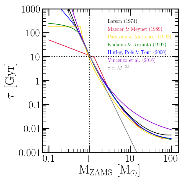
The total lifetimes of stars as a function of initial mass for the various forms recognized by VICE: Larson (1974; black), Maeder & Meynet (1989; red), Padovani & Matteucci (1993; yellow), Kodama & Arimoto (1997; green), Hurley, Pols & Tout (2000; blue), Vincenzo et al. (2016; purple), and the single power-law relationship (grey; see above). For the forms which take into account the metallicity-dependence of stellar lifetimes (Kodama & Aritmoto 1997; Hurley, Pols & Tout 2000; Vincenzo et al. 2016), the relationship is shown at solar metallicity. Those that compute main sequence lifetimes only as opposed to total lifetimes (all except Kodama & Arimoto 1997 and Vincenzo et al. 2016) are calculated with \(p_\text{MS}\) = 0.1 (i.e. the inferred total lifetimes are plotted for all forms).
3.2. The Cumulative Return Fraction
The cumulative return fraction is defined as the mass fraction of a single stellar population that is returned back to the interstellar medium (ISM) as gas. When dying stars produce their remnants, whatever material that does not end up in the remnant is returned to the ISM. This quantity can be calculated from an initial-final mass relation and an adopted stellar initial mass function (IMF). In short, the cumulative return fraction can be stated mathematically as “ejected material from dead stars in units of total initial amount of material.” Its analytic form is therefore given by:
The current version of VICE employs the initial-final remnant mass relation of Kalirai et al. (2008) [17]:
For a power-law IMF \(dN/dm \sim m^{-\alpha}\), the numerator of \(r(t)\) is thus given by:
for \(m_\text{to}(t) \geq 8\), and
for \(m_\text{to}(t) < 8\).
This solution is analytic. For piecewise IMFs, this becomes a summation over the relevant mass ranges of the IMF, and each term has the exact same form. The normalization of the IMF is irrelvant here, because the same normalization will appear in the denominator.
The denominator has a simpler analytic form:
Here we plot \(r\) as a function of the stellar population’s age assuming the mass-lifetime relation of Hurley, Pols & Tout (2000) [18] (see discussion here). Weinberg, Andrews, and Freudenburg (2017) [19] adopted instantaneous recycling, whereby a fraction of the stellar population’s mass \(r_\text{inst}\) is returned instantaneously in the interest of an analytic approach to singlezone models. They find that \(r_\text{inst}\) = 0.4 and \(r_\text{inst}\) = 0.2 is an adequate approximation for Kroupa [20] and Salpeter [21] IMFs. This reduces the more sophisticated formulation implemented here to:
In reality, the rate of mass return from a stellar population of mass \(M_*\) is given by \(\dot{r}M_*\), but in implementation, the quantization of timesteps allows each timestep to represent a single stellar population which will eject mass \(M_*dr\) in a time interval \(dt\). For that reason, VICE is implemented with a calculation of \(r(t)\) rather than \(\dot{r}\).
In simulations, VICE allows users the choice between the time-dependent formulation of \(r(t)\) derived here and the instantaneous approximation of Weinberg, Andrews, and Freudenburg (2017) by specifying a preferred value of \(r_\text{inst}\), which allows any fraction between 0 and 1.
In calculations of \(r(t)\) with the built-in Kroupa and Salpeter IMFs, the analytic solution is calculated. In the case of a user-customized IMF, VICE solves the equation numerically using quadrature with the methods described in chapter 4 of Press, Teukolsky, Vetterling & Flannery (2007) [22].
Note
The approximation of \(h(t) \approx 1 - r(t)\) where \(h\) is the main sequence mass fraction fails at the \(\sim5-10\%\) level. See our discussion of this point here.
Relevant source code:
vice/src/ssp/crf.c
vice/src/yields/integral.c
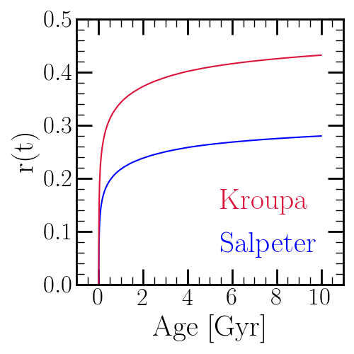
The cumulative return fraction as a function of age for Kroupa [23] (red) and Salpeter [24] (blue) IMFs assuming the mass-lifetime relation of Hurley, Pols & Tout (2000) [25] (see discussion here). The Kroupa IMF is higher at all nonzero ages because it has fewer low mass stars than Salpeter. In both cases the post main sequence lifetime is assumed to be 10% of the main sequence lifetime (i.e. \(p_\text{MS} = 0.1\)).
3.3. The Main Sequence Mass Fraction
The main sequence mass fraction, as the name suggests, is the fraction of a single stellar population’s initial mass that is still in the form of main sequence stars. Because this calculation does not concern evolved stars, neither a model for the post main sequence lifetime nor an initial-final remnant mass relation is needed; it is thus considerably simpler than the cumulative return fraction. This quantity is instead specified entirely by the IMF and the mass-lifetime relation.
It’s analytic form is given by:
which for a power-law IMF \(dN/dm \sim m^{-\alpha}\) becomes
It may be tempting to cancel the factor of \(1/(2 - \alpha)\), but more careful consideration must be taken for piece-wise IMFs like Kroupa [26]:
where the summation is over the relevant mass ranges with different power-law indeces \(\alpha_i\). In the case of kroupa \(\alpha\) = 2.3, 1.3, and 0.3 for \(m\) > 0.5, 0.08 \(\leq m \leq\) 0.5, and \(m\) < 0.08, respectively.
Here we plot \(h\) as a function of the stellar population’s age assuming the mass-lifetime relation of Hurley, Pols & Tout (2000) [27] (see discussion here). By 10 Gyr, \(h(t)\) is as low as \(\sim0.45\) for the Kroupa IMF and \(\sim0.65\) for the Salpeter [28] IMF. In comparison, the cumulative return fraction \(r(t) \approx 0.45\) for the Kroupa IMF and \(\sim0.28\) for the Salpeter IMF. This suggests that the approximation \(h(t) \approx 1 - r(t)\) fails at the \(\sim5-10\%\) level, depending on the choice of IMF. This suggests that for old stellar populations, a non-negligible portion of the mass is contained in evolved stars and stellar remnants. VICE therefore differentiates between these two quantities in its implementation.
In reality, the rate of the stellar mass evolving off of the main sequence is given by \(\dot{h}M_*\) where \(M_*\) is the initial mass of the stellar population. However, the quantization of timesteps in VICE allows each timestep to represent a single stellar population which will eject mass \(M_*dh\) in a time interval \(dt\). For that reason, VICE is implemented with a calculation of \(h(t)\) rather than \(\dot{h}\).
In calculations of \(h(t)\) with the built-in Kroupa and Salpeter IMFs, the analytic solution is calculated. In the case of a user-customized IMF, VICE solves the equation numerically using quadrature with the methods described in chapter 4 of Press, Teukolsky, Vetterling & Flannery (2007) [29].
Relevant source code:
vice/src/ssp/msmf.c
vice/src/yields/integral.c
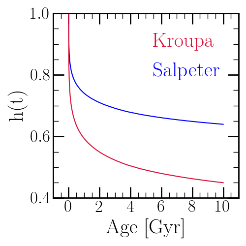
The main sequence mass fraction as a function of age for Kroupa [30] and Salpeter [31] IMFs assuming the mass-lifetime relation of Hurley, Pols & Tout (2000) [32] (see discussion here). The Kroupa IMF is lower at all nonzero ages because it has fewer low mass stars than Salpeter.
3.4. Enrichment from Single Stellar Populations
While galaxies form stars continuously, it is often an interesting scientific problem to quantify the nucleosynthetic production of only one population of conatal stars. This is inherently cheaper computationally, since this is only one stellar population while galaxy simulations require many stellar populations.
VICE includes functionality for simulating the mass production of a given element from a single stellar population (i.e. an individual star cluster) of given mass and metallicity under user-specified yields. This by construction does not take into account depletion from infall low metallicity gas and star formation, ejection in outflows, recycling, etc. It only calculates the mass production of the element as a function of the stellar population’s age.
The star cluster is assumed to form at time \(t = 0\), and thus at this time there is no net production. Because VICE operates under the assumption that all core-collapse supernovae (CCSNe) occur instantaneously following the star cluster’s formation [33], the entire CCSN net yield is injected within the first timestep at \(t = \Delta t\):
where \(y_x^\text{CC}(Z)\) is the user’s current setting for CCSN yields at a stellar metallicity Z. At subsequent timesteps, enrichment from asymptotic giant branch (AGB) stars is injected according to [34]:
and from type Ia supernovae (SN Ia) according to [35]:
These are the same equations that are implemented in simulating enrichment under the single-zone approximation, but applied to only one episode of star formation.
Users can run these simulations by calling vice.single_stellar_population.
Relevant Source Code:
vice/src/ssp/ssp.c
vice/core/ssp/_ssp.pyx
3.5. In Multizone Models
Like the timesteps in singlezone simulations, VICE treats star particles in multizone simulations as stand-ins for entire stellar populations. They eject newly produced heavy nuclei to the interstellar medium and recycle mass at their birth metallicities at the rates detailed in this section, where \(M_\star\) denotes the mass of the star particle.