2. Implementation
2.1. Motivation
VICE is designed in such a manner that as few assumptions as possible are made by the software itself. In this manner, the power the user has over the parameters of their simulations is maximized. With this motivation, any quantities that may vary are allowed to do so under user-constructed functions in Python. The only assumption VICE’s model adopts is physical plausibility.
2.2. Numerical Approach
Because VICE is built to handle singlezone and multizone simulations, numerics are not the dominant source of error, but rather in the model itself. The assumption of instantaneous diffusion of newly produced metals introduces an error that which is larger than even modest numerical errors to the equations presented in this documentation.
For this reason, VICE is implemented with a Forward Euler timestep solution, and its errors are not dominated by numerics. Furthermore, quantization of the timesteps allows the quantization of the episodes of star formation with no further assumptions. At several instances in this documentation, this will simplify the equations considerably. Adopting a user-specified timestep size, this also makes it the computationally cheapest solution by not introducing intermediate timesteps. In this manner, VICE is able to achieve a high degree of generality while retaining powerful computing speeds.
2.3. Minimization of Dependencies
VICE is implememented entirely in ANSI/ISO C and standard library Python and Cython. For this reason, it is highly portable across platforms and is independent of the user’s version of Anaconda (or lackthereof). However, VICE is not wrapped for installation in a Windows environment, and the developers do not provide support for non-POSIX operating systems. We therefore recommend that Windows users install and run VICE entirely within the Windows Subsystem for Linux.
2.4. Timed Runs
Due to the Forward Euler implementation and the requirement to calculate enrichment from previous episodes of star formation, we expect the integration time to scale with the square of the number of timesteps (i.e. \(T \propto (T_\text{end}/\Delta t)^2)\). VICE also treats each element independently and equally; the equations of enrichment are evaluated for an arbitrary element \(x\). The integration time should thus scale linearly with the number of elements \(N\).
Because VICE was implemented with the scientific motivation of studying the
enrichment of oxygen, iron, and strontium under starburst evolutionary
scenarios (Johnson & Weinberg 2020 [1]), the first integrations were ran
with these three elements. With timesteps of \(\Delta t\) = 1 Myr, each
simulation finished in 20.4 seconds on a system with a processing speed of
2.7 GHz. With these proportionalities and this calibration, we expect the
following scaling relation to describe the time per integration of the
singlezone object as a function of the number of elements \(N\), the
end time \(T_\text{end}\), and the timestep size \(\Delta t\):
Because 1 Myr is a relatively fine timestep, most integrations will typically not take this long. The default timestep size of 10 Myr is expected to finish in 68 milliseconds per element.
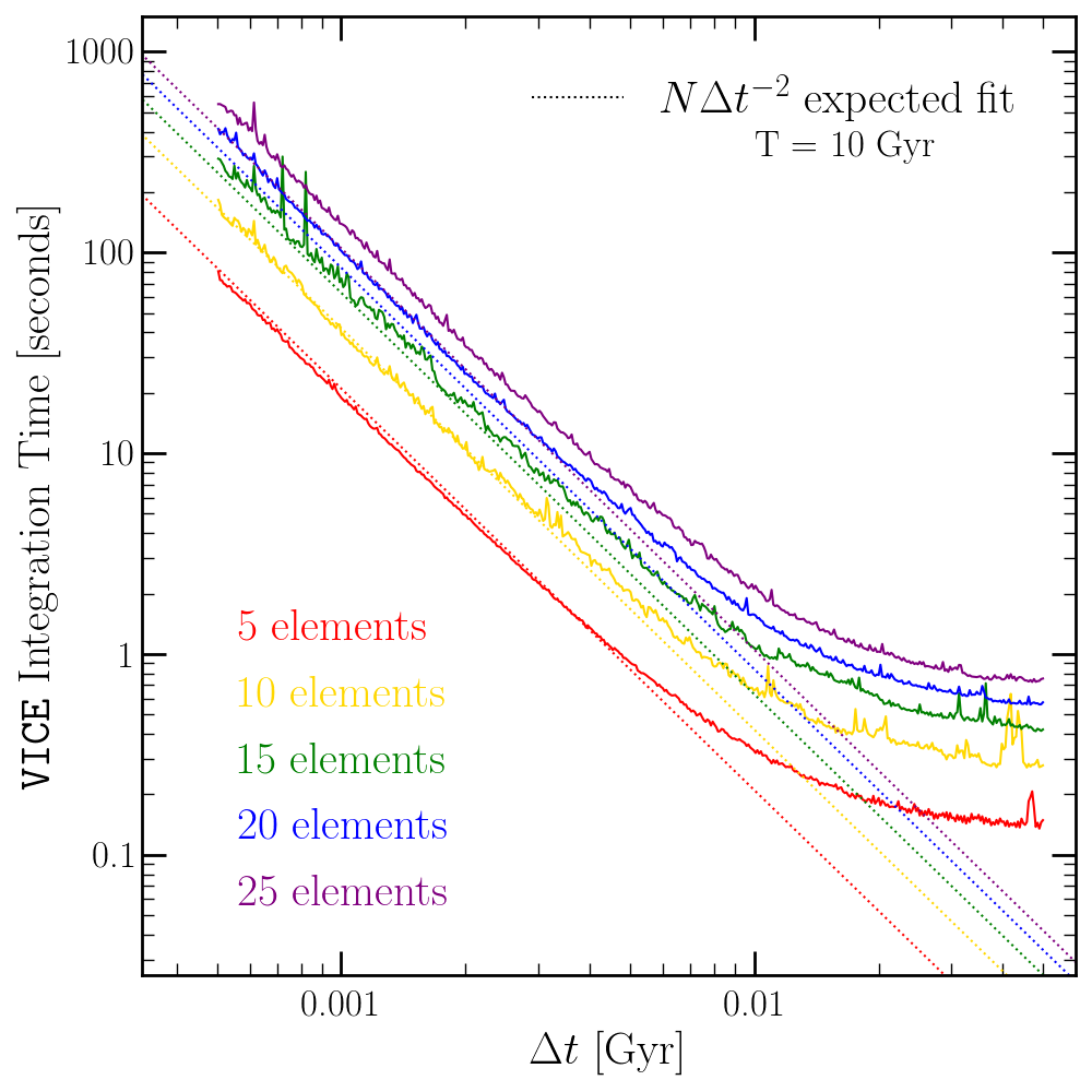
Timed runs with \(N\) = 5, 10, 15, 20, and 25 elements with timesteps ranging from 500 kyr to 10 Myr (solid lines) with an ending time of \(T_\text{end}\) = 10 Gyr. The color-coded dotted lines show the \(N\Delta t^{-2}\) expected scaling relation. The fit does well for small \(\Delta t\), but underpredicts the integration time for coarse timestepping; this is due to the transition from an algorithm limited simulation to a write out limited simulation. The scaling relation also slightly underpredicts the integration time for high N simulations.
Here we plot the integration time for 5, 10, 15, 20, and
25 elements with timesteps ranging from 500 kyr to 10 Myr in comparison to the
expected scaling relation in one-zone models with the singlezone object.
For small \(\Delta t\), the scaling relation describes the integration time
with sufficient accuracy, although slightly underpredicts the integration time
when the number of elements is large. This also underpredicts the integration
time for coarse timestepping; this is
because this scaling relation does not take into account write-out time. For
large \(\Delta t\), the singlezone object is not algorithm limited
but write-out limited. Write out time may also be a potential reason that
the integration time is mildly underpredicted for small \(\Delta t\) and
high \(N\).